Optimizing Chemical Reactions with Deep Reinforcement Learning
ACS Cent. Sci., 2017, 3 (12), pp 1337–1344

Overview
There has been various efforts on applying the idea of machine learning and artificial intelligence on the field of physical science. In terms of chemistry or biological science, some of the major interests are:
- Predictions disease states by applying classification / regression models on experimental data.
- Using a neural network to theoretically predict properties of molecules. And, one step further, to design new molecules.
- Predict the product of a reaction. And retro-synthesis analysis.
In this post, I will briefly introduction a recent work of applying the decision-making framework to solve real world problems in chemistry, specifically chemical reactions.
Common Ways to Optimize Chemical Reactions
There have been various attempts to use automated algorithms to optimize chemical reactions. For example:
- Nelder-Mead Simplex Method
- Stable Noisy Optimization by Branch and Fit (SNOBFIT)
Unfortunately, the most common practice among chemist to optimize a reaction is the one variable at a time (OVAT) method, which is changing a single experimental condition at a time while fixing all the others. This method often miss the optimal condition.
Our method
Problem Formulation
A reaction can be viewed as a system taking multiple inputs (experimental conditions) and providing one desired output. Example inputs include temperature, solvent composition, pH, catalyst, and time. Example outputs include product yield, selectivity, purity, and cost. The reaction can be modeled by a function $r = R(s)$, where $s$ stands for the experimental conditions and $r$ denotes the objective, say, the yield.
There are two properties makes optimizing chemical reactions a hard problem:
chemical reactions are expensive and time-consuming to conduct
the outcome can vary largely, which is caused in part by measurement errors.
A Decision-Making Framwork
We can formulate the process of finding the optimal reaction condition as a decision making problem, i.e., a Markov decision process (MDP) of $(\mathcal{S}, \mathcal{A}, \{P_{sa}\}, \mathcal{R})$:
$\mathcal{S}$ denotes the set of states $s$. In the context of reaction optimization, $\mathcal{S}$ is the set of all possible combinations of experimental conditions.
$\mathcal{A}$ denotes the set of actions $a$. In the context of reaction optimization, $\mathcal{A}$ is the set of all changes that can be made to the experimental conditions, for example, increasing the temperature by 10 °C and so forth.
$ \{P_{sa} \} $ denotes the state transition probabilities. Concretely, $P_{sa}$ specifies the probability of transiting from $s$ to another state with action $a$. In the context of a chemical reaction, $P_{sa}$ specifies to what experimental conditions the reaction will move if we decide to make a change a to the experimental condition $s$. Intuitively, $P_{sa}$ measures the inaccuracy when operating the instrument. For example, the action of increasing the temperature by 10 °C may result in a temperature increase of 9.5–10.5 °C.
$\mathcal{R}$ denotes the reward function of state $s$ and action $a$. In the environment of a reaction, the reward $r$ is only a function of state $s$, i.e., a certain experimental condition $s$ (state) is mapped to yield $r$ (reward) by the reward function $r = R(s)$.
Our goal is to find a policy for this decision making problem. In the context of chemical reactions, the policy refers to the algorithm that interacts with the chemical reaction to obtain the current reaction condition and reaction yield, from which the next experimental conditions are chosen. Rigorously, we define the policy as the function $\pi$, which maps from the current experimental condition $s_t$ and history of the experiment record $\mathcal{H}_t$ to the next experimental condition, that is,
$$ s_{t+1} = \pi (s_t,\mathcal{H}_t)$$
where $\mathcal{H}_t$ is the history, and $t$ records the number of steps we have taken in reaction optimization.
Here, we use a different defination of policy compared to the traditional one of $a = \pi (s)$. This is for simplicity and it has no conflict with the traditional policy defination, because in chemical reaction, we can define the action as the vector difference between two states: $a_t = s_{t+1} - s_t$.
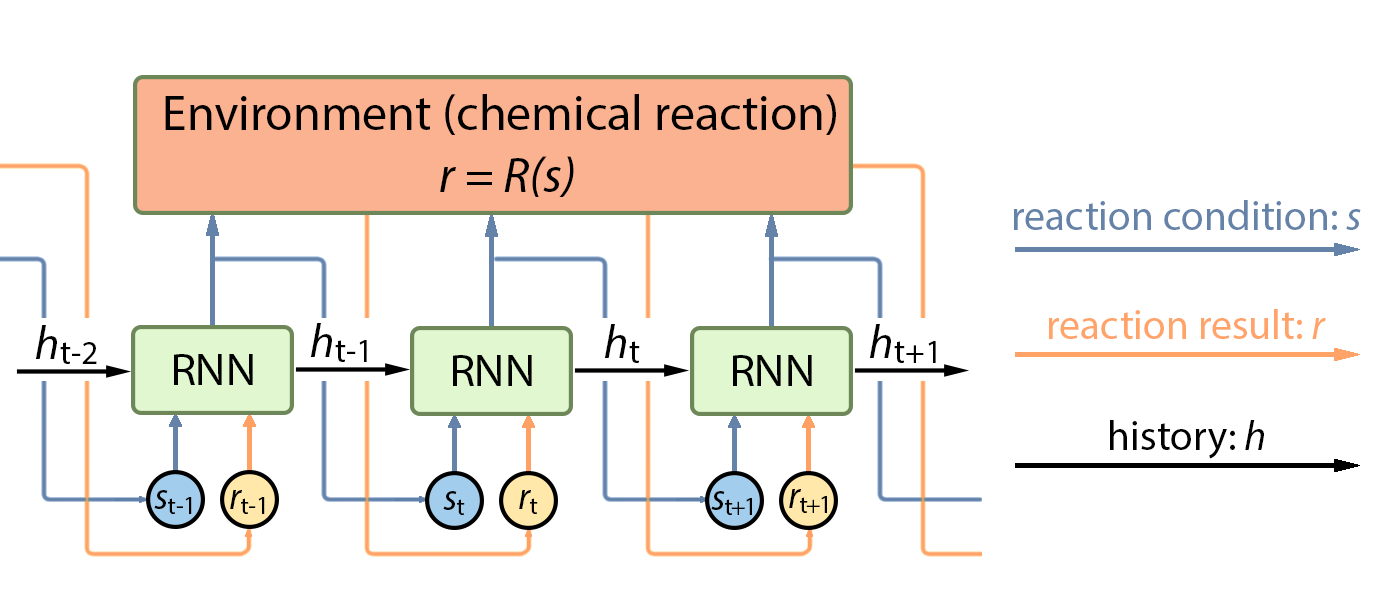
Intuitively, the optimization procedure can be explained as follows: We iteratively conduct an experiment under a specific experimental condition and record the yield. Then the policy function makes use of all the history of experimental record (what condition led to what yield) and tells us what experimental condition we should try next. This procedure is illustrated in Figure 1.
Recurrent Neural Network as Policy
We employs the recurrent neural network (RNN) to fit the policy function $\pi$ under the settings of chemical reactions. A RNN takes a similar form of the policy function can be written as follows:
$$s_{t+1},h_{t+1}=\mathrm{RNN}_\theta(s_t,r_t,h_t)$$
where at time step $t$, $h_t$ is the hidden state to model the history $\mathcal{H}_t$, $s_t$ denotes the state of reaction condition, and $r_t$ is the yield (reward) of reaction outcome. The policy of RNN maps the inputs at time step $t$ to outputs at time step $t + 1$.
And the loss function is defined as the observed improvement:
$$l(\theta) = -\sum_{t=1}^{T}\left(r_t-\max_{i<t}r_i\right)$$
The term inside the parentheses measures the improvement we can achieve by iteratively conducting different experiments. The loss function encourages reaching the optimal condition faster, in order to address the problem that chemical reactions are expensive and time-consuming to conduct.
Results
Simulated Reactions
As mentioned earlier, chemical reactions are time-consuming to evaluate. Although our model can greatly accelerate the procedure, we still propose to first train the model on simulated reactions. A set of mixture Gaussian density functions is used as the simulated reactions environment $r = R(s)$. A Gaussian error term is added to the function to model the large variance property of chemical reaction measurements. The mock reactions can be written as:
$$ y = \sum_{i=1}^N c_i (2\pi)^{-k/2}|\Sigma_i|^{-1/2} \exp\left(-\frac{1}{2}(x-\mu_i)^T\Sigma_i^{-1}(x-\mu_i)\right) +\varepsilon$$
where $c_i$ is the coefficient, $\mu_i$ is the mean, and $\Sigma_i$ is the covariance of a multivariate Gaussian distribution; $k$ is the dimension of the variables. $\varepsilon$ is the error term, which is a random variable drawn from a Gaussian distribution with mean $0$ and variance $\sigma^2$.
The motivation for using a mixture of Gaussian density functions comes from the idea that they can be used to approximate arbitrarily close all continuous functions on a bounded set. We assume that the response surface for most reactions is a continuous function, which can be well approximated by a mixture of Gaussian density functions. Besides, a mixture of Gaussian density functions often has multiple local minima. The rationale behind this is that the response surface of a chemical reaction may also have multiple local optima. As a result, we believe a mixture of Gaussian density functions can be a good class of function to simulate real reactions.
We compared our model with several state-of-the-art blackbox optimization algorithms of covariance matrix adaption–evolution strategy (CMA-ES), Nelder–Mead simplex method, and stable noisy optimization by branch and fit (SNOBFIT) on another set of mixture Gaussian density functions that are unseen during training. This comparison is a classic approach for model evaluation in machine learning. We use “regret” to evaluate the performance of the models. The regret is defined as
$$ \mathrm{regret}(t) = \max_s R(s) - r_t$$
and it measures the gap between the current reward and the largest reward that is possible. Lower regret indicates better optimization.
Figure 2A shows the average regret versus time steps of the two algorithms from which we see that our model outperforms CMA-ES significantly by reaching a lower regret value in fewer steps.
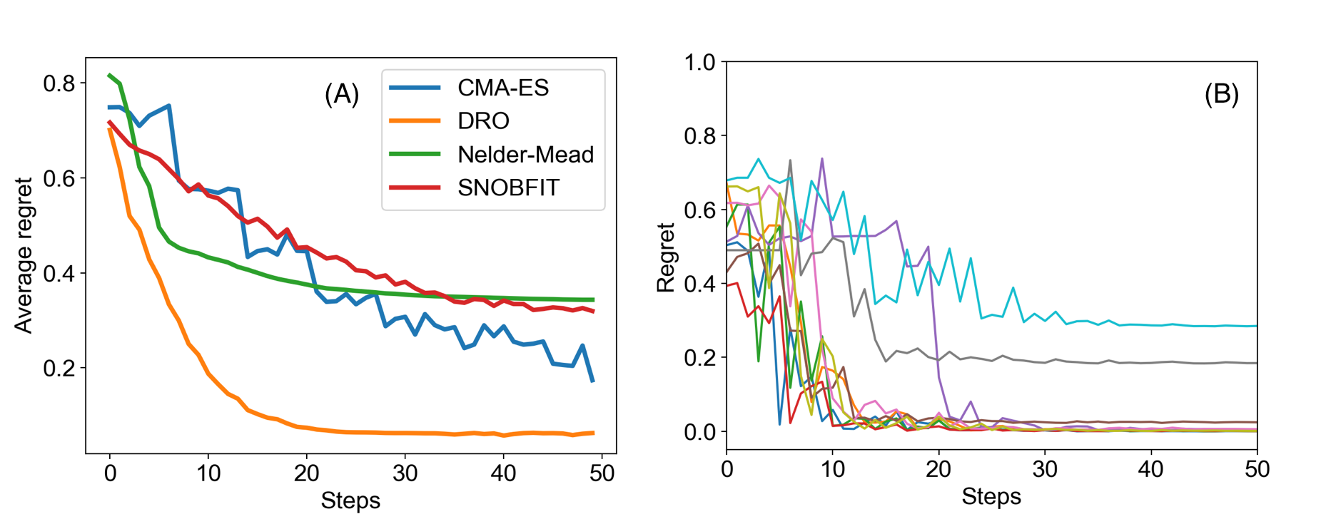
Randomized Policy for Deep Exploration
Although our model optimizes nonconvex functions faster than CMA-ES, we observe that it sometimes get stuck in a local maximum (Figure 2B) because of the deterministic greedy policy, where greedy means making the locally optimal choice at each stage without exploration. In the context of reaction optimization, a greedy policy will stick to one reaction condition if it is better than any other conditions observed. However, the greedy policy will get trapped in a local optimum, failing to explore some regions in the space of experimental conditions, which may contain a better reaction condition that we are looking for. To further accelerate the optimization procedure in this aspect, we proposed a randomized exploration regime to explore different experimental conditions, in which randomization means drawing the decision randomly from a certain probability distribution. This idea came from the work of Van Roy and co-workers, which showed that deep exploration can be achieved from randomized value function estimates. The stochastic policy also addresses the problem of randomness in chemical reactions.
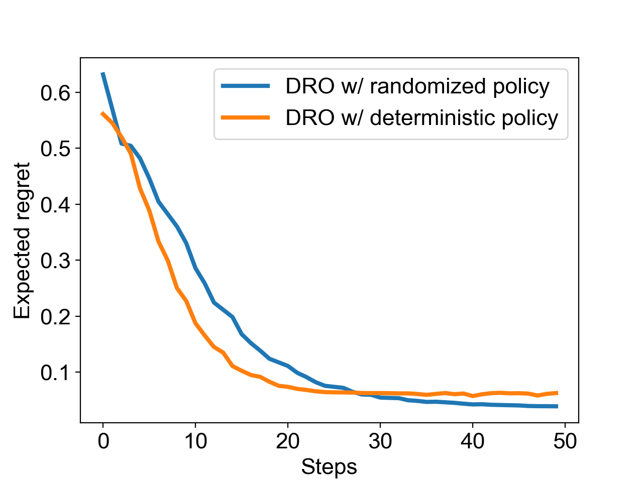
A stochastic recurrent neural network was used to model a randomized policy, which can be written as
$$s_{t+1}\sim\mathcal{N}\left(\mu_{t+1},\Sigma_{t+1}\right)$$
Similar to the notations introduced before, the RNN is used to generate the mean $\mu_{t+1}$, and the covariance matrix $\Sigma_{t+1}$; the next state $s_{t+1}$ is then drawn from a multivariate Gaussian distribution of $\mathcal{N}(\mu_{t+1},\Sigma_{t+1})$ at time step $t + 1$. This approach achieved deep exploration in a computationally efficient way.
Figure 3 compares between the greedy policy and the randomized policy on another group of simulated reactions. Although the randomized policy was slightly slower, it arrives to a better function value owing to its more efficient exploration strategy. Comparing the randomized policy with a deterministic one, the average regret was improved from 0.062 to 0.039, which shows a better chance of finding the global optimal conditions.
Optimization of Real Reactions
We carried out four experiments in microdroplets and recorded the production yield: The Pomeranz–Fritsch synthesis of isoquinoline, Friedländer synthesis of a substituted quinoline, the synthesis of ribose phosphate, and the reaction between 2,6-dichlorophenolindophenol (DCIP) and ascorbic acid. Our model outperformed the other two methods by reaching a higher yield in fewer steps. In both reactions, the model found the optimal condition within 40 steps, with the total time of 30 min required to optimize a reaction. (Figure 4)
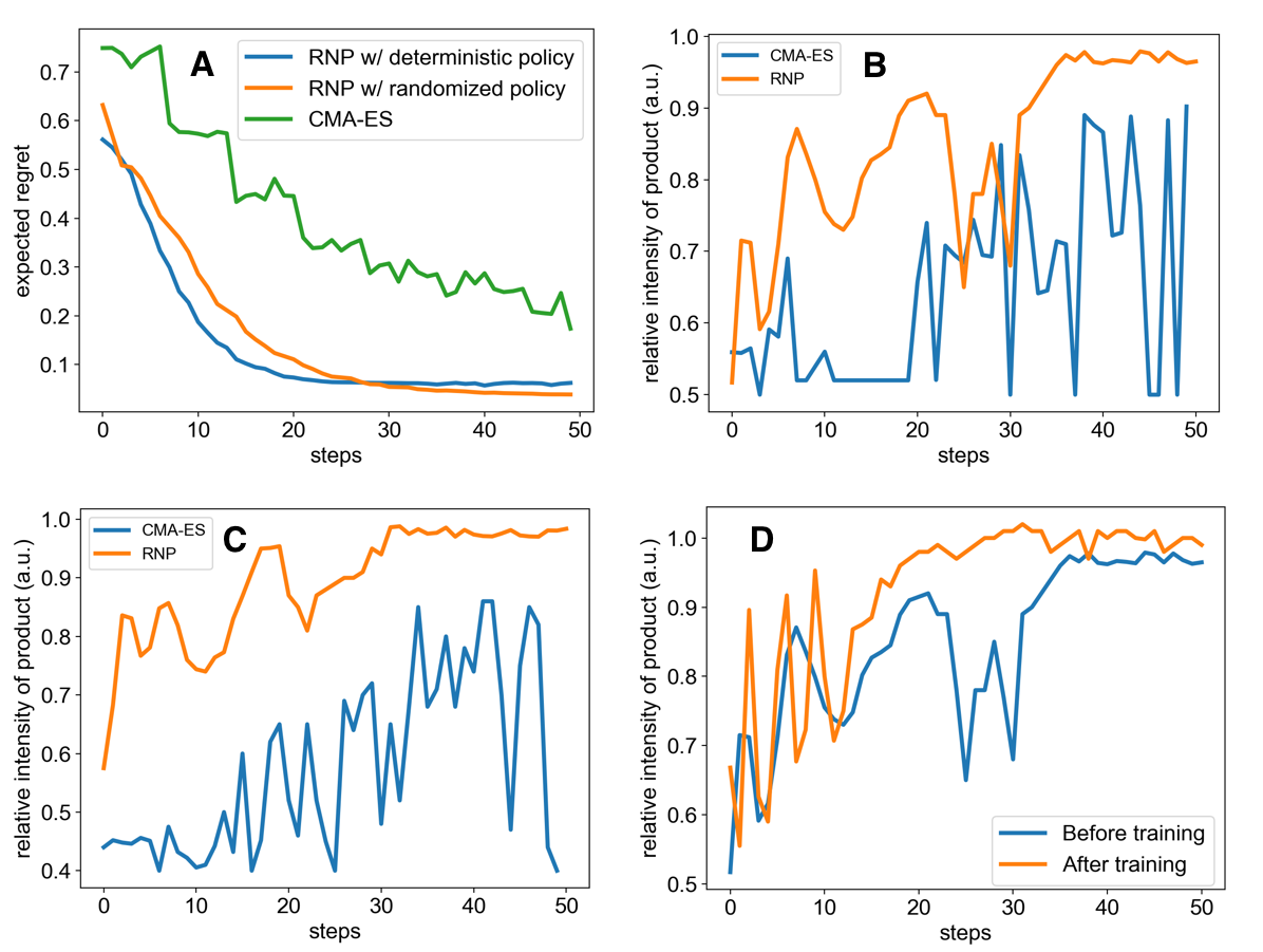
Learning for Better Optimization
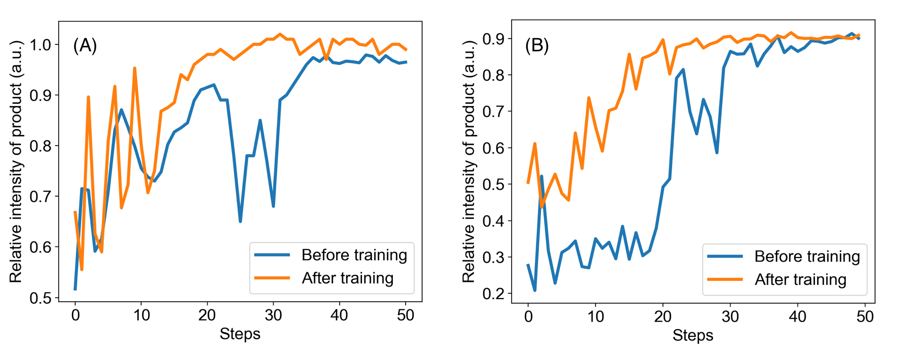
We also observed that the algorithm is capable of learning while optimizing on real experiments. In other words, each time running a similar or even dissimilar reactions will improve the policy. To demonstrate this point, the model was first trained on the reaction of the Pomeranz–Fritsch synthesis of isoquinoline and then tested on the reaction of the Friedländer synthesis of substituted quinoline. Figure 5 compares the performance of the model before and after training. The policy after training showed a better performance by reaching a higher yield at a faster speed.
Conclusion
Our model showed strong generalizability in two ways: First, based on optimization of a large family of functions, our optimization goal can be not only yield but also selectivity, purity, or cost, because all of them can be modeled by a function of experimental parameters. Second, a wide range of reactions can be accelerated by $10^3$ to $10^6$ times in microdroplets. Showing that a microdroplet reaction can be optimized in 30 min by our model, we therefore propose that a large class of reactions can be optimized by our model. The wide applicability of our model suggests it to be useful in both academic research and industrial production.
Code Availability
The code of this project can be found here